\(\renewcommand\AA{\unicode{x212B}}\)

Indirect Data Reduction¶

Table of Contents

Overview ¶

The Indirect Data Reduction interface provides the initial reduction that is used to convert raw instrument data to S(Q, w) for analysis in the Indirect Data Analysis and Indirect Bayes interfaces.

The tabs shown on this interface will vary depending on the current default facility such that only tabs that will work with data from the facility are shown, this page describes all the tabs which can possibly be shown.

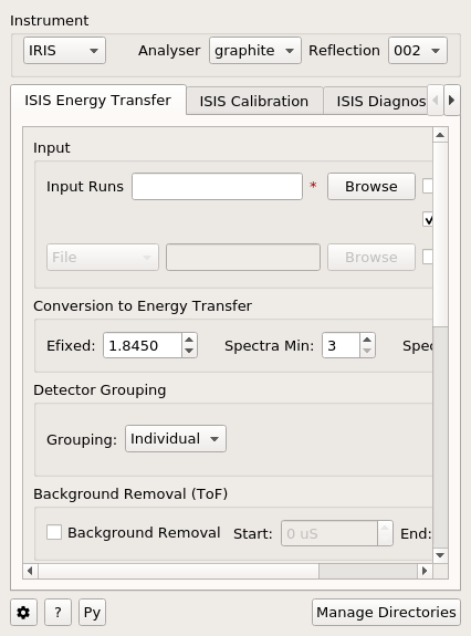
../../_images/Data_Reduction_interface.png

Instrument Options ¶

Instrument: Used to select the instrument on which the data being reduced was created on.
Analyser: The analyser bank that was active when the experiment was run, or for which you are interested in seeing the results of.
Reflection: The reflection plane of the instrument set up.

Tip

If you need clarification as to the instrument setup you should use please speak to the instrument scientist who dealt with your experiment.

Action Buttons ¶

Settings: Opens the Settings GUI which allows you to customize the settings for the Indirect interfaces.

?: Opens this help page.
Py: Exports a Python script which will replicate the processing done by the current tab.
Manage Directories: Opens the Manage Directories dialog allowing you to change your search directories and default save directory and enable/disable data archive search.

ISIS/ILL Energy Transfer ¶

If the default facility has been set to ISIS, then the ISIS Energy Transfer tab will be available. However, this tab will be replaced by the ILL Energy Transfer tab if the default facility has been set to ILL. A further explanation of each tab can be found below.

ISIS Energy Transfer ¶

This tab provides you with the functionality to convert the raw data from the experiment run into units of \(\Delta E\). See the algorithm ISISIndirectEnergyTransfer.

ISIS Energy Transfer Options ¶

Input Runs: Allows you to select the raw data files for an experiment. You can enter these either by clicking on the Browse button and selecting them, or entering the run numbers. Multiple files can be selected, multiple run numbers can be separated by a comma (,) or a range can be specified by using a dash (-).
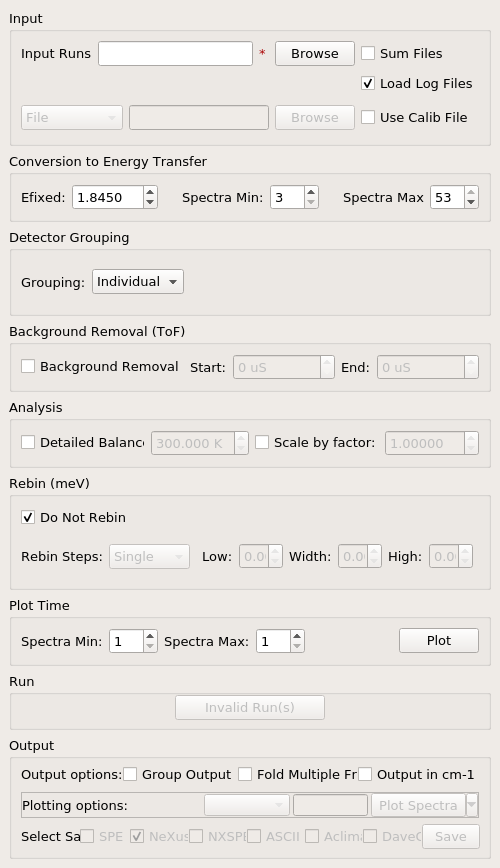
Sum Files: If selected the data from each raw file will be summed and from then on treated as a single run.
Load Log Files: If selected the sample logs will be loaded from each of the run files.
Use Calib File & Calibration File: Allows you to select a calibration file created using the Calibration tab.
Efixed: This option allows you to override the default fixed final energy for the analyser and reflection number setting. This can be useful in correcting an offset peak caused by the sample being slightly out of centre.
Spectra Min/Spectra Max: Used to specify a range of spectra.
Detector Grouping: Used to specify a method for grouping spectra. Possible grouping options include Individual, All, File, Groups and Custom. The TOSCA instrument also has the Default grouping option which will use the grouping specified in the IPF.
Background Removal: Allows removal of a background given a time-of-flight range.
Detailed Balance: Gives the option to perform an exponential correction on the data once it has been converted to Energy based on the temperature. This is automatically loaded from the sample logs of the input file if available.
Scale by Factor: Gives the option to scale the output by a given factor.
Do Not Rebin: If selected it will disable the rebinning step.
Rebin Steps: Select the type of rebinning you wish to perform.
Plot Time: Creates a time of flight plot of the grouping of the spectra in the range defined in the Plot Time section. To include a single spectrum, set the Spectra Min and Spectra Max selectors to the same value. Note that this first rebins the sample input to ensure that each detector spectrum has the same binning in order to be grouped into a single spectrum.
Spectra Min & Spectra Max: Select the range of detectors you are interested in, default values are chosen based on the instrument and analyser bank selected.
Run: Runs the processing configured on the current tab.
Plot Spectra: If enabled, it will plot the selected workspace indices in the selected output workspace.
Plot Contour: If enabled, it will plot the selected output workspace as a contour plot.
Group Output: This will place the output reduced files from a reduction into a group workspace.
Fold Multiple Frames: This option is only relevant for TOSCA. If checked, then multiple-framed data will be folded back into a single spectra, if unchecked the frames will be left as is with the frame number given at the end of the workspace name.
Output in \(cm^{-1}\): Converts the units of the energy axis from \(meV\) to wave number (\(cm^{-1}\)).
Select Save Formats: Allows you to select multiple output save formats to save the reduced data as, in all cases the file will be saved in the default save directory.

ISIS Energy Transfer Example Workflow ¶

The ISIS Energy Transfer tab operates on raw TOF data files. Before starting this workflow, go to Manage Directories and make sure that Search Data Archive is set to all.

Set the Instrument to be OSIRIS, the Analyser to be graphite and the Reflection to be 002.
In Input Runs, enter the run numbers 104371-104375 and press enter.
Change the Spectra Min and Spectra Max if you want to avoid some of the detectors. For the purposes of this demonstration, keep them at their default values.
The Detector Grouping option allows you to specify how you want to group your detectors. The different option available are explained in the Grouping section. For this demonstration, choose Individual.
Click Run and wait for the interface to finish processing. This should generate a workspace ending in _red.
Choose a default save directory and then tick the Nexus checkbox. Click Save to save the output workspace. The workspace ending in _red will be used in the Elwin Example Workflow.

Go to the ISIS Calibration Example Workflow.

Grouping ¶

The following options are available for grouping output data:

Custom

Follows the same grouping patterns used in the GroupDetectors algorithm. An example of the syntax is 1,2+3,4-6,7:10

This would produce spectra for: spectra 1, the sum of spectra 2 and 3, the sum of spectra 4-6 (4+5+6) and individual spectra from 7 to 10 (7,8,9,10)

Individual

All detectors will remain on individual spectra.

Groups

The detectors will automatically be divided into a given number of equal size groups. Any left over will be added as an additional group.

All

All detectors will be grouped into a single spectra.

File

Gives the option of supplying a grouping file to be used with the GroupDetectors algorithm.

Default

This grouping option is only available for TOSCA. It uses the spectra grouping specified in the IPF.

Rebinning ¶

Rebinning can be done using either a single step or multiple steps as described in the sections below.

Single: In this mode only a single binning range is defined as a range and width.

../../_images/Data_Reduction_pgSingleRebin_widget.png

Multiple: In this mode multiple binning ranges can be defined using the rebin string syntax used by the Rebin algorithm.

../../_images/Data_Reduction_pgMultipleRebin_widget.png

A note on Masked Detectors ¶

When a reduction of a single run number takes place, the masked detectors used for the reduction are found using the IdentifyNoisyDetectors algorithm.

When using the Sum Files option the noisy detectors for each of the run numbers could be different. In this case, the masked detectors for the summed run is found by first finding the noisy detectors for each of the individual runs within the summed run using IdentifyNoisyDetectors. For instance, let us say that we find that the following run numbers have these noisy detectors:

Run number 22841 has noisy detectors 53, 54, 55
Run number 22842 has noisy detectors 53, 54, 56
Run number 22843 has noisy detectors 53, 55, 56

To find the detectors which should be masked for a summed run of 22841-22843 we first combine these noisy detectors so that we have 53, 54, 55 and 56. A summed file is then calculated from these run numbers and the IdentifyNoisyDetectors algorithm finds the noisy detectors for this summed file.

Summed file 22841-22843 has noisy detectors 13, 53, 54, 55

The masked detectors used for the summed run would also include any additional detectors found to be noisy for the summed run. The masked detectors used for the summed reduction of 22841-22843 would therefore be 13, 53, 54, 55 and 56.

ILL Energy Transfer ¶

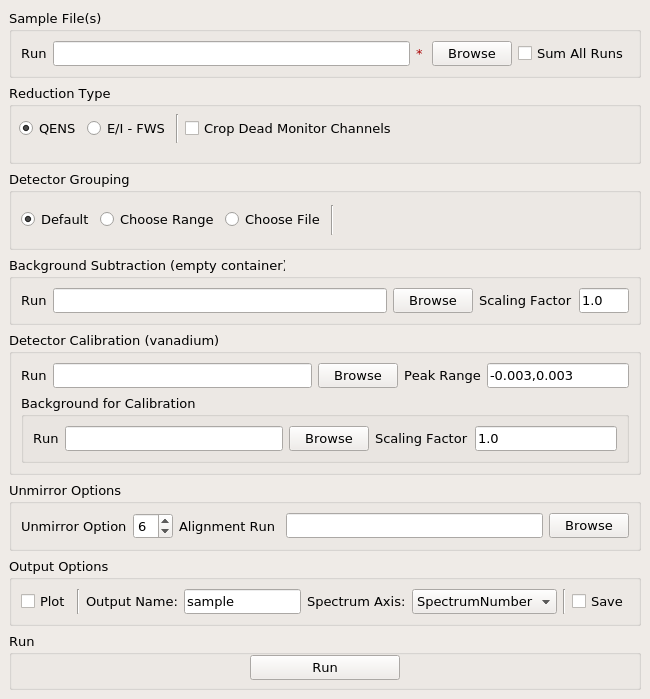
This tab handles the reduction of data from the IN16B instrument and will appear when the default facility is set to be the ILL. See the algorithm IndirectILLEnergyTransfer.

Reduction Type ¶

There are two reduction types of IN16B data: Quasi-Elastic Neutron Scattering (QENS) or Fixed Window Scans (FWS). The latter can be either Elastic (EFWS) or Inelastic (IFWS). If one or another reduction type is checked, the corresponding algorithm will be invoked (see IndirectILLReductionQENS and IndirectILLReductionFWS). There are several properties in common between the two, and several others that are specific to one or the other. The specific ones will show up or disappear corresponding to the choice of the reduction type.

Common Options ¶

Input File: Used to select the raw data in .nxs format. Note that multiple files can be specified following MultipleFileProperty instructions.
Detector Grouping: Used to switch between grouping as per the IDF (Default) or grouping using a mapping file (Map File). This defines e.g. the summing of the vertical pixels per PSDs.
Background Subtraction: Used to specify the background (i.e. empty can) runs to subtract. A scale factor can be applied to background subtraction.
Detector Calibration: Used to specify the calibration (i.e. vanadium) runs to divide by.
Background Subtraction for Calibration: Used to specify the background (i.e. empty can) runs to subtract from the vanadium calibration runs.
Output Name: This will be the name of the resulting reduced workspace group.
Spectrum Axis: This allows the spectrum axis to be converted to elastic momentum transfer or scattering angle if desired.
Plot: If enabled, it will plot the result (of the first run) as a contour plot.
Save: If enabled the reduced workspace group will be saved as a .nxs file in the default save directory.

QENS-only Options ¶

Sum All Runs: If checked, all the input runs will be summed while loading.
Crop Dead Monitor Channels: If checked, the few channels in the beginning and at the end of the spectra that contain zero monitor counts will be cropped out. As a result, the doppler maximum energy will be mapped to the first and last non-zero monitor channels, resulting in narrower peaks. Care must be taken with this option; since this alters the total number of bins, problems might occur while subtracting the background or performing unmirroring if the number of dead monitor channels are different.
Calibration Peak Range: This defines the integration range over the peak in calibration run in meV.
Unmirror Options: This is used to choose the option of summing of the left and right wings of the data, when recorded in mirror sense. See IndirectILLReductionQENS for full details. Unmirror option 5 and 7 require vanadium alignment run.

FWS-only Options ¶

Observable: This is the scanning observable, that will become the x-axis of the final result. It can be any numeric sample parameter defined in Sample Logs (e.g. sample.*) or a time-stamp string (e.g. start_time). It can also be the run number. It can not be an instrument parameter.
Sort X Axis: If checked, the x-axis of the final results will be sorted.
Sum/Interpolate: Both background and calibration have options to use the summed (averaged) or interpolated values over different observable points. Default behaviour is Sum. Interpolation is done using cubic (or linear for 2 measured values only) splines. If interpolation is requested, x-axis will be sorted automatically.

ISIS Calibration ¶

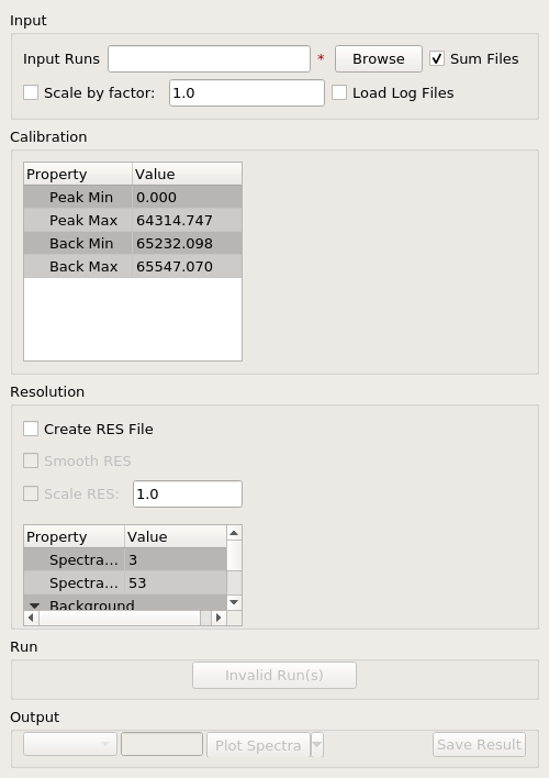
This tab gives you the ability to create Calibration and Resolution files, and is only available when the default facility is set to ISIS.

The calibration file is normalised to an average of 1.

../../_images/Data_Reduction_tabISISCalibration_widget.png

ISIS Calibration Options ¶

Input Runs: This allows you to select a run for the function to use, either by selecting the .raw file with the Browse button or through entering the number in the box.
Plot Raw: Updates the preview plots.
Intensity Scale Factor: Optionally applies a scale by a given factor to the raw input data.
Load Log Files: This will load the log files if enabled.
Run: Runs the processing configured on the current tab.
Plot Spectra: If enabled, it will plot the selected workspace indices in the selected output workspace.
Plot Bins: If enabled, it will plot the selected bin indices in the selected output workspace.
Save Result: If enabled the result will be saved as a NeXus file in the default save directory.

Calibration ¶

Peak Min & Peak Max: Selects the time-of-flight range corresponding to the peak. A default starting value is generally provided from the instrument’s parameter file.
Back Min & Back Max: Selects the time-of-flight range corresponding to the background. A default starting value is generally provided from the instrument’s parameter file.

Resolution ¶

Create RES File: If selected, it will create a resolution file when the tab is run.
Smooth RES: If selected, the WienerSmooth algorithm will be applied to the output of the resolution algorithm.
Scale RES: Applies a scale by a given factor to the resolution output.
Spectra Min & Spectra Max: Allows restriction of the range of spectra used when creating the resolution curve.
Background Start & Background End: Defines the time-of-flight range used to calculate the background noise.
Low, Width & High: Binning parameters used to rebin the resolution curve.

Options ¶

Input Files: File for the calibration (e.g. vanadium) run. If multiple specified, they will be automatically summed.
Grouping: Used to switch between grouping as per the IDF (Default) or grouping using a mapping file (Map File).
Peak Range: Sets the integration range over the peak in \(meV\)
Scale Factor: Factor to scale the intensities with

ISIS Calibration Example Workflow ¶

The ISIS Calibration tab operates on raw TOF data files. Before starting this workflow, go to Manage Directories and make sure that Search Data Archive is set to all.

Set the Instrument to be IRIS, the Analyser to be graphite and the Reflection to be 002.
In Input Runs, enter the run number 26176 and press enter.
Tick Create RES File. This will create a workspace ending in _res.
Click Run and wait for the interface to finish processing. This should generate workspaces ending in _red, _res and _calib. The calibration workspace can be used in the ISIS Energy Transfer tab by ticking Use Calib File.
Select the workspace ending in _calib in the output options. Enter index 0 in the neighbouring box, and then click the down arrow on the Plot Spectra button, and select Plot Bins. This will plot the bin at index 0.
Select the workspace ending in _res in the output options. Enter index 0 in the neighbouring box, and then click the Plot Spectra button. This will plot the spectrum at workspace index 0.
Choose a default save directory and then click Save Result to save the workspaces ending in _res and _calib. The _res file is used in the I(Q, t) Example Workflow and ConvFit Example Workflow. The _calib file is used in the ISIS Diagnostics Example Workflow.

ISIS Diagnostics ¶

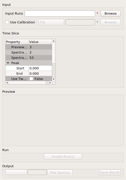
This tab allows you to perform an integration on a raw file over a specified time of flight range, and is equivalent to the Slice functionality found in MODES. It is only available when the default facility is set to ISIS.

ISIS Diagnostics Options ¶

Input Runs: This allows you to select a run for the function to use, either by selecting the .raw file with the Browse button or through entering the number in the box. Multiple files can be selected, in the same manner as described for the Energy Transfer tab.
Use Calibration: Allows you to select either a calibration file or workspace to apply to the raw files.
Preview Spectrum: Allows selection of the spectrum to be shown in the preview plot to the right of the Time Slice section.
Spectra Min & Spectra Max: Allows selection of the range of detectors you are interested in, this is automatically set based on the instrument and analyser bank that are currently selected.
Peak: The time-of-flight range that will be integrated over to give the result (the blue range in the plot window). A default starting value is generally provided from the instrument’s parameter file.
Use Two Ranges: If selected, enables subtraction of the background range.
Background: An optional range denoting background noise that is to be removed from the raw data before the integration is performed. A default starting value is generally provided from the instrument’s parameter file.
Run: Runs the processing configured on the current tab.
Plot Spectra: If enabled, it will plot the selected workspace indices in the selected output workspace.
Save Result: If enabled the result will be saved as a NeXus file in the default save directory.

ISIS Diagnostics Example Workflow ¶

The ISIS Diagnostics tab operates on raw TOF data files. Before starting this workflow, go to Manage Directories and make sure that Search Data Archive is set to all.

Set the Instrument to be IRIS, the Analyser to be graphite and the Reflection to be 002.
In Input Runs, enter the run number 26176 and press enter.
Tick Use Calibration and load the file named irs26173_graphite002_calib.
Change the Preview Spectrum variable to view a different spectrum in the mini-plot.
Change the Start and End variables to specify a PeakRange for the TimeSlice algorithm. Alternatively, you can move the blue sliders on the mini-plot.
Click Run and wait for the interface to finish processing. This should generate a workspace ending in _slice. The Preview mini-plot will be updated.
Click Plot Spectra to produce a larger plot of the Preview mini-plot.

Go to the Transmission Example Workflow.

Transmission ¶

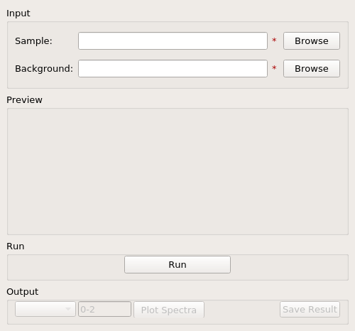
Calculates the sample transmission using the raw data files of the sample and its background or container. The incident and transmission monitors are converted to wavelength and the transmission monitor is normalised to the incident monitor over the common wavelength range. The sample is then divided by the background/container to give the sample transmission as a function of wavelength.

Transmission Options ¶

Sample: Allows the selection of a raw file to be used as the sample.
Background: Allows the selection of a raw file to be used as the background.
Run: Runs the processing configured on the current tab.
Plot Spectra: If enabled, it will plot the selected spectra indices in the selected output workspace.
Save Result: If enabled the result will be saved as a NeXus file in the default save directory.

Transmission Example Workflow ¶

The Transmission tab operates on raw TOF data files. Before starting this workflow, go to Manage Directories and make sure that Search Data Archive is set to all.

Set the Instrument to be IRIS, the Analyser to be graphite and the Reflection to be 002.
In the Sample box, enter the run number 26176 and press enter. In the Background box, enter the run number 26174 and press enter.
Click Run and wait for the interface to finish processing. This will run the algorithm IndirectTransmissionMonitor and plots the output workspaces in the Preview mini-plot.
Click Plot Spectra to produce a larger plot of the Preview mini-plot.

Go to the Symmetrise Example Workflow.

Symmetrise ¶

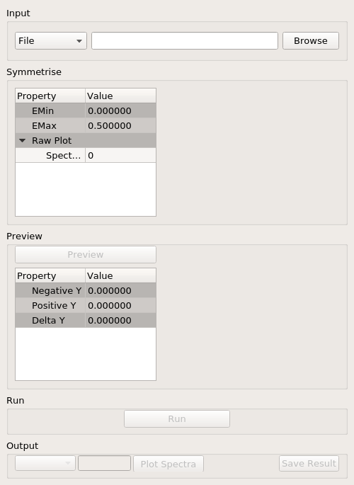
This tab allows you to take an asymmetric reduced file (_red.nxs) and symmetrise it about the Y axis.

The curve is symmetrised such that the range of positive values between \(EMin\) and \(EMax\) are reflected about the Y axis and replaces the negative values in the range \(-EMax\) to \(-EMin\), the curve between \(-EMin\) and \(EMin\) is not modified.

../../_images/Data_Reduction_tabSymmetrise_widget.png

Symmetrise Options ¶

Input: Allows you to select a reduced NeXus file (_red.nxs) or workspace (_red) as the input to the algorithm.
EMin & EMax: Sets the energy range that is to be reflected about \(y=0\).
Spectrum No: Changes the spectrum shown in the preview plots.
XRange: Changes the range of the preview plot, this can be useful for inspecting the curve before running the algorithm.
Preview: This button will update the preview plot and parameters under the Preview section.
Run: Runs the processing configured on the current tab.
Plot Spectra: If enabled, it will plot the selected workspace indices in the selected output workspace.
Save Result: If enabled the result will be saved as a NeXus file in the default save directory.

Preview ¶

The preview section shows what a given spectra in the input will look like after it has been symmetrised and gives an idea of how well the value of EMin fits the curve on both sides of the peak.

Negative Y: The value of \(y\) at \(x=-EMin\).
Positive Y: The value of \(y\) at \(x=EMin\).
Delta Y: The difference between Negative and Positive Y. Typically this should be as close to zero as possible.

Symmetrise Example Workflow ¶

The Symmetrise tab operates on _red files. The file used in this workflow can be produced using the 26176 run number on the ISIS Energy Transfer tab. The instrument used to produce this file is IRIS, the analyser is graphite and the reflection is 002. See the ISIS Energy Transfer Example Workflow.

In the Input box, load the file named iris26176_graphite002_red. This will automatically plot the data on the first mini-plot.
Move the green slider located at x = -0.5 to be at x = -0.4.
Click Preview. This will update the Preview properties and the neighbouring mini-plot.
Click Run and wait for the interface to finish processing. This will run the Symmetrise algorithm. The output workspace is called iris26176_graphite002_sym_red.
Click Plot Spectra to produce a spectra plot of the output workspace. Other indices can be plotted by entering indices in the box next to the Plot Spectra button. For example, entering indices 0-2,4,6-7 will plot the spectra with workspace indices 0, 1, 2, 4, 6 and 7.

Go to the S(Q, w) Example Workflow.

S(Q, w)¶

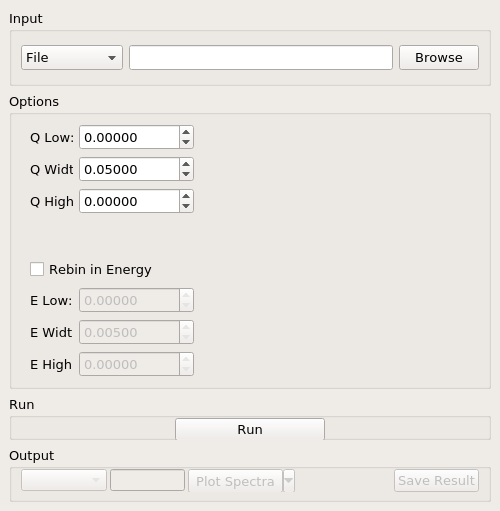
Provides an interface for running the SofQW algorithm.

../../_images/Data_Reduction_tabSQw_widget.png

S(Q, w) Options ¶

Input: Allows you to select a reduced NeXus file (_red.nxs) or workspace (_red) as the input to the algorithm. An automatic contour plot of _rqw will be plotted in the preview plot once a file has finished loading.
Q Low, Q Width & Q High: Q binning parameters that are passed to the SofQW algorithm. The low and high values can be determined using the neighbouring contour plot.
Rebin in Energy: If enabled the data will first be rebinned in energy before being passed to the SofQW algorithm.
E Low, E Width & E High: The energy rebinning parameters. The low and high values can be determined using the neighbouring contour plot.
Run: Runs the processing configured on the current tab.
Plot Spectra: If enabled, it will plot the selected workspace indices in the selected output workspace.
Plot Contour: If enabled, it will plot the selected output workspace as a contour plot.
Save Result: If enabled the result will be saved as a NeXus file in the default save directory.

S(Q, w) Example Workflow ¶

The S(Q, w) tab operates on _red files. The file used in this workflow can be produced using the 26176 run number on the ISIS Energy Transfer tab. The instrument used to produce this file is IRIS, the analyser is graphite and the reflection is 002. See the ISIS Energy Transfer Example Workflow.

In the Input box, load the file named iris26176_graphite002_red. This will automatically plot the data as a contour plot within the interface.
Set the Q Low, Q Width and Q High to be 0.5, 0.05 and 1.8. These values are read from the contour plot.
Tick Rebin in Energy.
Set the E Low, E Width and E High to be -0.5, 0.005 and 0.5. Again, these values should be read from the contour plot.
Click Run and wait for the interface to finish processing. This will perform an energy rebin before performing the SofQW algorithm. The output workspace ends with suffix _sqw and is called iris26176_graphite002_sqw.
Enter a list of workspace indices in the output options (e.g. 0-2,4,6-7) and then click Plot Spectra to plot spectra from the output workspace.

Click the down arrow on the Plot Spectra button, and select Plot Contour. This will produce a contour plot of the output workspace.
Choose a default save directory and then click Save Result to save the output workspace. The _sqw file is used in the Moments Example Workflow.

Moments ¶

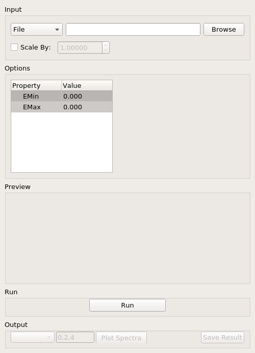
This interface uses the SofQWMoments algorithm to calculate the \(n^{th}\) moment of an \(S(Q, \omega)\) workspace created by the SofQW tab.

Moments Options ¶

Input: Allows you to select an \(S(Q, \omega)\) file (_sqw.nxs) or workspace (_sqw) as the input to the algorithm.
Scale By: Used to set an optional scale factor by which to scale the output of the algorithm.
EMin & EMax: Used to set the energy range of the sample that the algorithm will use for processing.
Run: Runs the processing configured on the current tab.
Plot Spectra: If enabled, it will plot the selected workspace indices in the selected output workspace.
Save Result: If enabled the result will be saved as a NeXus file in the default save directory.

Moments Example Workflow ¶

The Moments tab operates on _sqw files. The file used in this workflow is produced during the S(Q, w) Example Workflow.

In the Input box, load the file named irs26176_graphite002_sqw. This will automatically plot the data in the first mini-plot.
Drag the blue sliders on the mini-plot so they are x=-0.4 and x=0.4.
Click Run and wait for the interface to finish processing. This will run the SofQWMoments algorithm. The output workspace ends with suffix _moments and is called iris26176_graphite002_moments.

Categories: Interfaces | Indirect